=SUM(data)/COUNT(data)
= n p
=
=
=

| Statistic | Equations | Excel |
|---|---|---|
| Sample size | n | = COUNT(data) |
| Population size | N | |
| Sample mean | =AVERAGE(data) =SUM(data)/COUNT(data) |
|
| Formulas for the population mean m | = x P(x) = n p |
|
| Sample Standard Deviation | = sx = |
=STDEV(data) |
| Population Standard Deviation | = = = |
|
| Slope | =SLOPE(y data, x data) | |
| Intercept | =INTERCEPT(y data, x data) | |
| Correlation | =CORREL(y data, x data) | |
| Binomial probability | = nCr pr q(n-r) | =COMBIN(n,r)*p^r*q^(n-r) |
| Calculate a z value from an x | z = |
=STANDARDIZE(x, m, s) |
| Calculate an x value from a z | x = s z + m | |
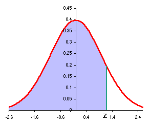
| Calculate a cumulative probability from a z value where the probability is calculated from negative infinity to z. | =NORMSDIST(z) | |
| Calculate a z value from a probability where the probability is calculated from negative infinity to z. | =NORMSINV(probability) | |
| Calculate a z value from an |
 |
=STANDARDIZE(x, m, s/SQRT(n)) |
DHL has found that the delivery time for packages is normally distributed with mean 14 hours and standard deviation 2 hours.
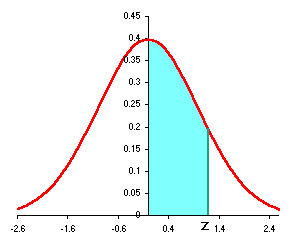
Table of standard normal probabilities from 0 to z. For values of z larger than 2.69 use 0.497.
| 0.00 | 0.01 | 0.02 | 0.03 | 0.04 | 0.05 | 0.06 | 0.07 | 0.08 | 0.09 | |
|---|---|---|---|---|---|---|---|---|---|---|
| 0.0 | 0.000 | 0.004 | 0.008 | 0.012 | 0.016 | 0.020 | 0.024 | 0.028 | 0.032 | 0.036 |
| 0.1 | 0.040 | 0.044 | 0.048 | 0.052 | 0.056 | 0.060 | 0.064 | 0.067 | 0.071 | 0.075 |
| 0.2 | 0.079 | 0.083 | 0.087 | 0.091 | 0.095 | 0.099 | 0.103 | 0.106 | 0.110 | 0.114 |
| 0.3 | 0.118 | 0.122 | 0.126 | 0.129 | 0.133 | 0.137 | 0.141 | 0.144 | 0.148 | 0.152 |
| 0.4 | 0.155 | 0.159 | 0.163 | 0.166 | 0.170 | 0.174 | 0.177 | 0.181 | 0.184 | 0.188 |
| 0.5 | 0.191 | 0.195 | 0.198 | 0.202 | 0.205 | 0.209 | 0.212 | 0.216 | 0.219 | 0.222 |
| 0.6 | 0.226 | 0.229 | 0.232 | 0.236 | 0.239 | 0.242 | 0.245 | 0.249 | 0.252 | 0.255 |
| 0.7 | 0.258 | 0.261 | 0.264 | 0.267 | 0.270 | 0.273 | 0.276 | 0.279 | 0.282 | 0.285 |
| 0.8 | 0.288 | 0.291 | 0.294 | 0.297 | 0.300 | 0.302 | 0.305 | 0.308 | 0.311 | 0.313 |
| 0.9 | 0.316 | 0.319 | 0.321 | 0.324 | 0.326 | 0.329 | 0.331 | 0.334 | 0.336 | 0.339 |
| 1.0 | 0.341 | 0.344 | 0.346 | 0.348 | 0.351 | 0.353 | 0.355 | 0.358 | 0.360 | 0.362 |
| 1.1 | 0.364 | 0.367 | 0.369 | 0.371 | 0.373 | 0.375 | 0.377 | 0.379 | 0.381 | 0.383 |
| 1.2 | 0.385 | 0.387 | 0.389 | 0.391 | 0.393 | 0.394 | 0.396 | 0.398 | 0.400 | 0.401 |
| 1.3 | 0.403 | 0.405 | 0.407 | 0.408 | 0.410 | 0.411 | 0.413 | 0.415 | 0.416 | 0.418 |
| 1.4 | 0.419 | 0.421 | 0.422 | 0.424 | 0.425 | 0.426 | 0.428 | 0.429 | 0.431 | 0.432 |
| 1.5 | 0.433 | 0.434 | 0.436 | 0.437 | 0.438 | 0.439 | 0.441 | 0.442 | 0.443 | 0.444 |
| 1.6 | 0.445 | 0.446 | 0.447 | 0.448 | 0.449 | 0.451 | 0.452 | 0.453 | 0.454 | 0.454 |
| 1.7 | 0.455 | 0.456 | 0.457 | 0.458 | 0.459 | 0.460 | 0.461 | 0.462 | 0.462 | 0.463 |
| 1.8 | 0.464 | 0.465 | 0.466 | 0.466 | 0.467 | 0.468 | 0.469 | 0.469 | 0.470 | 0.471 |
| 1.9 | 0.471 | 0.472 | 0.473 | 0.473 | 0.474 | 0.474 | 0.475 | 0.476 | 0.476 | 0.477 |
| 2.0 | 0.477 | 0.478 | 0.478 | 0.479 | 0.479 | 0.480 | 0.480 | 0.481 | 0.481 | 0.482 |
| 2.1 | 0.482 | 0.483 | 0.483 | 0.483 | 0.484 | 0.484 | 0.485 | 0.485 | 0.485 | 0.486 |
| 2.2 | 0.486 | 0.486 | 0.487 | 0.487 | 0.487 | 0.488 | 0.488 | 0.488 | 0.489 | 0.489 |
| 2.3 | 0.489 | 0.490 | 0.490 | 0.490 | 0.490 | 0.491 | 0.491 | 0.491 | 0.491 | 0.492 |
| 2.4 | 0.492 | 0.492 | 0.492 | 0.492 | 0.493 | 0.493 | 0.493 | 0.493 | 0.493 | 0.494 |
| 2.5 | 0.494 | 0.494 | 0.494 | 0.494 | 0.494 | 0.495 | 0.495 | 0.495 | 0.495 | 0.495 |
| 2.6 | 0.495 | 0.495 | 0.496 | 0.496 | 0.496 | 0.496 | 0.496 | 0.496 | 0.496 | 0.496 |
The above table shows the standard normal probability from 0 to z as seen at the left below. The Excel functions use left to z as shown at the right below.

