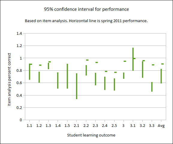
Chart one: 95% Confidence intervals for performance by SLO
The following document is based on the proposed outline. By using the outline as the basis for reporting assessment of learning, the document seeks to close the design-deploy-assess loop in a single document.
Course Description: A one semester course designed as an introduction to the basic ideas of data presentation, descriptive statistics, linear regression, and inferential statistics including confidence intervals and hypothesis testing. Basic concepts are studied using applications from education, business, social science, and the natural sciences. The course uses spreadsheet software for both data analysis and presentation.
| Deployed design | ↺ | Assessed result1 | ||||
|---|---|---|---|---|---|---|
| CLO | PLO 3.1 | PLO 3.2 | ↓ ↑ | CLO | PLO 3.1 | PLO 3.2 |
| 1 | I,D,M | I,D | 1 | 0.93 | 0.88 | |
| 2 | I,D | I | 2 | 0.82 | ||
| 3 | I,D | I,D,M | 3 | 0.94 | 0.99 | |
| Deployed design | ||
|---|---|---|
| CLO | PLO 3.1 | PLO 3.2 |
| 1 | 1.1 1.3 1.4 1.5 | 1.2 |
| 2 | 2.1 2.2 2.3 2.4 2.5 | 2.1 |
| 3 | 3.1 3.2 3.3 | 3.1 3.2 3.3 |
| Assessed result | |||
|---|---|---|---|
| CLO | SLO | PLO 3.1 | PLO 3.2 |
| CLO1 | 1.1 | 0.90 | |
| 1.2 | 0.91 | 0.88 | |
| 1.3 | 0.94 | ||
| 1.4 | |||
| 1.5 | |||
| CLO2 | 2.1 | ||
| 2.2 | 0.97 | ||
| 2.3 | 0.93 | ||
| 2.4 | 0.79 | ||
| 2.5 | 0.77 | ||
| CLO3 | 3.1 | 0.99 | 0.99 |
| 3.2 | 0.96 | ||
| 3.3 | 0.89 | ||
| Student learning outcomes | Assessment strategies | iA2 |
|---|---|---|
| 1.1 Identify levels of measurement and appropriate statistical measures for a given level | Quizzes and/or tests. | 0.90 |
| 1.2 Determine frequencies, relative frequencies, creating histograms and identifying their shape visually. | 0.89 | |
| 1.3 Calculate basic statistical measures of the middle, spread, and relative standing. | 0.94 | |
| 1.4 Calculate simple probabilities for equally likely outcomes. | NA | |
| 1.5 Determine the mean of a distribution. | NA |
| Student learning outcomes | Assessment strategies | iA |
|---|---|---|
| 2.1 Calculate probabilities using the normal distribution | Quizzes and/or tests. | NA |
| 2.2 Calculate the standard error of the mean | 0.97 | |
| 2.3 Find confidence intervals for the mean | 0.93 | |
| 2.4 Perform hypothesis tests against a known population mean using both confidence intervals and formal hypothesis testing | 0.79 | |
| 2.5 Perform t-tests for paired and independent samples using both confidence intervals and p-values | 0.77 |
| Student learning outcomes | Assessment strategies | iA |
|---|---|---|
| 3.1 Calculate the linear slope and intercept for a set of data | Quizzes and/or tests. | 0.99 |
| 3.2 Calculate the correlation coefficient r | 0.96 | |
| 3.3 Generate predicted values based on the regression | 0.89 |
Due to frequent power outages in the weeks prior to the final examination, a decision was made to run the final examination as a take-home test. The final examination has been an open book examination for four years. The reasoning is that no one takes away a statistician's texts and references and then asks the statistician to do their work. Although open book, the final examination has remained an individual effort performed in a two hour period proctored by the instructor.
This term the students were given three and half days to complete the final examination. Although students were asked to work on their examinations individually, there was no way to ensure students had not collaborated on the final examination, or at the minimum, had checked their answers against those of other students.
Overall, the result was a statistically significantly improved performance on almost all student learning outcomes that were measured by the final examination. Chart one depicts the 95% confidence intervals for the past performance as vertical lines. The horizontal lines are the performance on the current term take-home examination. The vertical access is the percentage success rate based on an item analysis of the final examination.

Chart one: 95% Confidence intervals for performance by SLO
Note that student learning outcomes 1.4, 1.5, and 2.1 were not covered by the final examination. In-class quizzes and tests measured those outcomes. As those quizzes and tests were not take-home tests, the results have been omitted above.
The take-home final examination resulted in a strongly improved performance on the final examination. Put another way, the performance was anomalously high against historic performance levels.
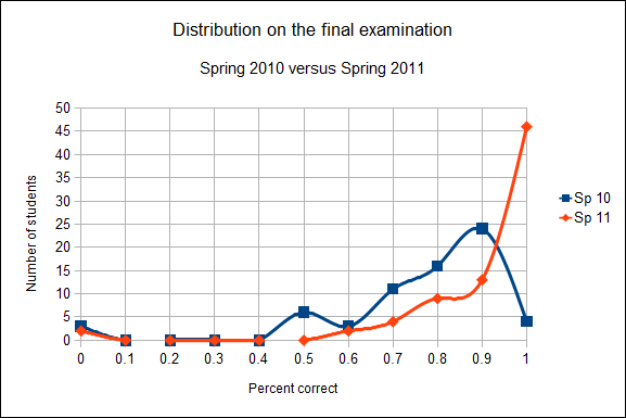
The performance gains on the take-home final examination are strongly evident in the distribution of scores. A comparison of the score distribution from spring 2010 against spring 2011 is provided in chart two. Spring 2010 was used for the comparison as the fall 2010 term final examination was structured differently.

Chart two: Student score distributions on the final examinations of spring 2010 and spring 2011.
While chart two clearly shows the improvement from an in-class to a take-home examination, of note is that the peak of the distribution moved up by only 10% from a 90% to a 100% peak.
The grade distribution spring 2011 is provided in the following table.
| Grade | Frequency | Relative Frequency |
|---|---|---|
| A | 46 | 0.61 |
| B | 13 | 0.17 |
| C | 11 | 0.14 |
| D | 2 | 0.03 |
| F | 2 | 0.03 |
| 0 | 2 | 0.03 |
As indicated in both the chart and table, 46 students correctly answered 90% or more of the questions on the spring 2011 take-home final examination. Bear in mind that the test was not specifically designed to be a take-home examination. The test paralleled previous final examinations in structure. Thus two students failing the exam outright and two others attaining a grade of D is somewhat surprising. Note that the two zeros were students who neither picked up nor turned in a final examination.
MS 150 Statistics had three sections that ran Monday, Wednesday, and Friday for an hour each at 8:00, 9:00, and 10:00. There were no statistically significant differences in gender or sections subgroups. The following table details average overall course performance by section and gender, none of the differences was found to be statistically significant. Performance values were slightly higher than the previous term, but not statistically significantly higher except in the overall average. The overall average improved from 77% to 83% in part due to the improved take-home final examination performance.
| Section | Female | Male | Section average |
|---|---|---|---|
| 8:00 | 0.82 | 0.81 | 0.82 |
| 9:00 | 0.85 | 0.78 | 0.83 |
| 10:00 | 0.85 | 0.85 | 0.85 |
| Averages: | 0.82 | 0.83 | Overall: 0.83 |
1Average percent of students demonstrating the learning outcome. Average may be based on multiple encounters with the outcome on the final examination.
2 iA is Assessed result and is based on item analysis of final examination.